Using a Faster R-CNN Deep Neural Network to Track Objects for the Sport of Roundnet.

A second look at sports analytics for the sport of roundnet

By: Austin Ulfers

Published: November 22nd, 2021

Background

Over the past year and a half, I have continued to be interested in the idea of developing a sports analytics pipeline for roundnet. Like how AWS is used in the NFL’s Next Gen Stat’s ecosystem [1], I believe something similar could be implemented and would be beneficial. In March of 2020, I set out to begin developing my attempt at a similar pipeline but aimed at the sport of roundnet instead of football.

Previous Document

A lot has changed between my first version [2] and the version presented here. There were quite a few limitations of the previous process, the main ones being that the footage was explicitly selected for the environment and the footage was gathered using a drone overtop of the game which is not a standard way to collect footage from a match.

Self Improvement

Since the release of that document, I have continued to improve on the methodology outlined there. The way I was going about finding and tracking the ball was very rudimentary and not easily generalizable to other videos. I knew that I would need a fundamental shift in how I was thinking about this problem. However, I did not have the skills necessary to act on it. At the time I was a Junior at the University of Washington with only a year and a half of experience with Python and had not taken all the machine learning classes available to me yet. Since then, I have graduated with my degree in Informatics with a specialization in data science, have a solid 3 years of programming experience with Python, and have several other computer vision projects under my belt.

Abstract

Within this document, I will outline the process for tracking a roundnet ball within a video using Facebook’s Detectron2 [3] Faster R-CNN model with transfer learning. Once objects within the video are established, a series of algorithm and machine learning operations are performed to determine the active ball within a video of a single roundnet round. Through these operations, generalizable tracking was successfully established but further work is needed to implement analytics tracking on a per-player basis.

Outline

This document will follow one video as we progress through the methodology. However, it should be noted that this process is generalizable to commonly gathered roundnet footage. Illustrations and captures of the process will be outlined along the way. Later in this document, I will cover the limitations as well as the recommendations for future iterations of these methods.

Introduction

Annotated Training Data

To begin, I would like to give a much needed thank you to the University of Washington husky roundnet club [4] for the donation of their footage archive to be used for the purpose of this project. They donated over 300 gigabytes of video footage from over 40 unique locations & lighting conditions.

Since my solution involved a Faster R-CNN object detection model with transfer learning [5], I knew that I would only need a small subset of images to train, validate, and test my model. To facilitate this, I created a couple helper functions to extract random images from the video library and spent roughly 12 hours labeling all images.

Every annotated image had objects of the following two classes:

• Net
• Ball

Roboflow

Before I wanted to dive into creating the object detection model on my own, I wanted to test and make sure that the annotations that I had could produce results capable of the time investment needed to develop the model. I chose to use Roboflow [6] as my proof-of-concept choice because it aims to commercialize the computer vision industry and it has a very low bar for entry. Below you can see the results from that training.

Overall:

mAP	precision	recall
93.5%	64.9%	94.8%

Although these results are great, they start to degrade when you look at the specific precision score for each class.

	Net	Ball
precision	94%	40%

The roboflow training graphs can be seen in Figure 1.

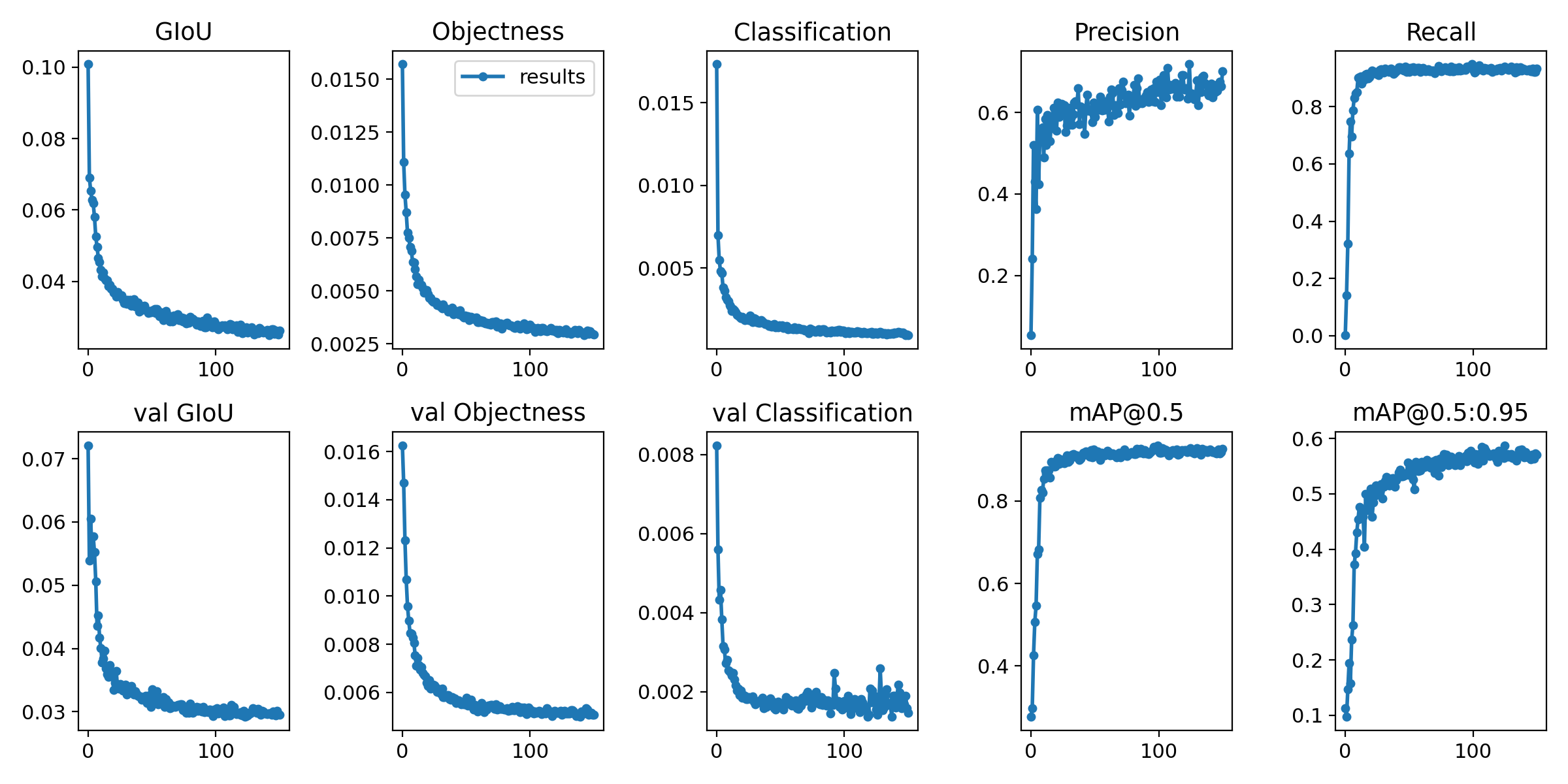Figure 1: Roboflow training graphs.

Although not perfect, this proved as a satisfactory proof of concept for me to continue with the project. After getting this done, I knew at some point in the future I would need to develop my own model because of the costs associated with Roboflow.

Per their pricing model, training credits are limited, and it costs $10 per 1000 inferences which is only a 33 second video so I knew I would need a cheaper solution.

After a lot of searching a lot of time spent trying to configure my development environment, I eventually got a detectron2 faster r-cnn model trained on my annotated dataset. It can take individual images and predict the locations of balls and Nets within the image. Some of the results from that training can be seen in Figure 2. I left a lot of the default values in for the training and didn’t do much hyperparameter tuning so I believe this model could be greatly improved in the future with more training data, and some better tuning.

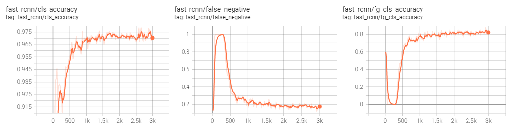
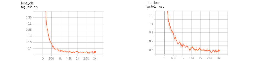
Figure 2: Various measurements from the detectron2 training of 3000 epochs.

This model turned out to be even more accurate than the Roboflow model which is also a plus. However, now that we have an accessible model, let’s move onto applying it.

Sample Video

Below is a low resolution gif of the sample video. However, a full resolution video can be found on YouTube here. https://www.youtube.com/watch?v=kgmbi1J97FA

Figure 3: Sample video in gif format.

This video is a part of my test set in which the model was not trained on any of these images so when the model predicts on these frames, it is seeing them for the first time. We will follow this video through the methodology that is outlined next.

Methodology

Inferencing

Now, the first step in order to track these objects is to complete inferencing on each of the video frames. Since the model that was used only works on individual images, it was necessary to divide the video up into frames. This is one area of potential improvement that will be discussed more at the bottom of this document.

After passing in the image to the model, we get an object that contains all the bounding box information for all the detected objects in the image.

A gif of the inferred video using the model can be seen below. Again, a higher resolution video can be found on YouTube here. https://www.youtube.com/watch?v=VIlFG7NpFNk. Anything with a blue bounding box is a roundnet ball and anything with a red bounding box is a Net.

Figure 4: Sampled video with object detection inferences.

As you can see within this video, there are multiple balls identified so the next problem becomes identifying the active ball.

Finding the Active Ball

After iterating on several different options of identification, I ended up landing on what I believe is a good generalizable solution that only operates under the following assumption.

• There is only one active ball within the span of the video.
• The ball that moves the most at the beginning is the active and all others are considered exclusionary.
• The active ball can be identified within the first 90 frames of the video.
• A ball will not be removed from an exclusionary position for the duration of the video.

To enforce these assumptions, I take the first 90 frames of the video and examine all ball positions over time. This gives a three-dimensional view where the X and Y axes are their respective pixel positions on the camera and the Z axis is the frame number.

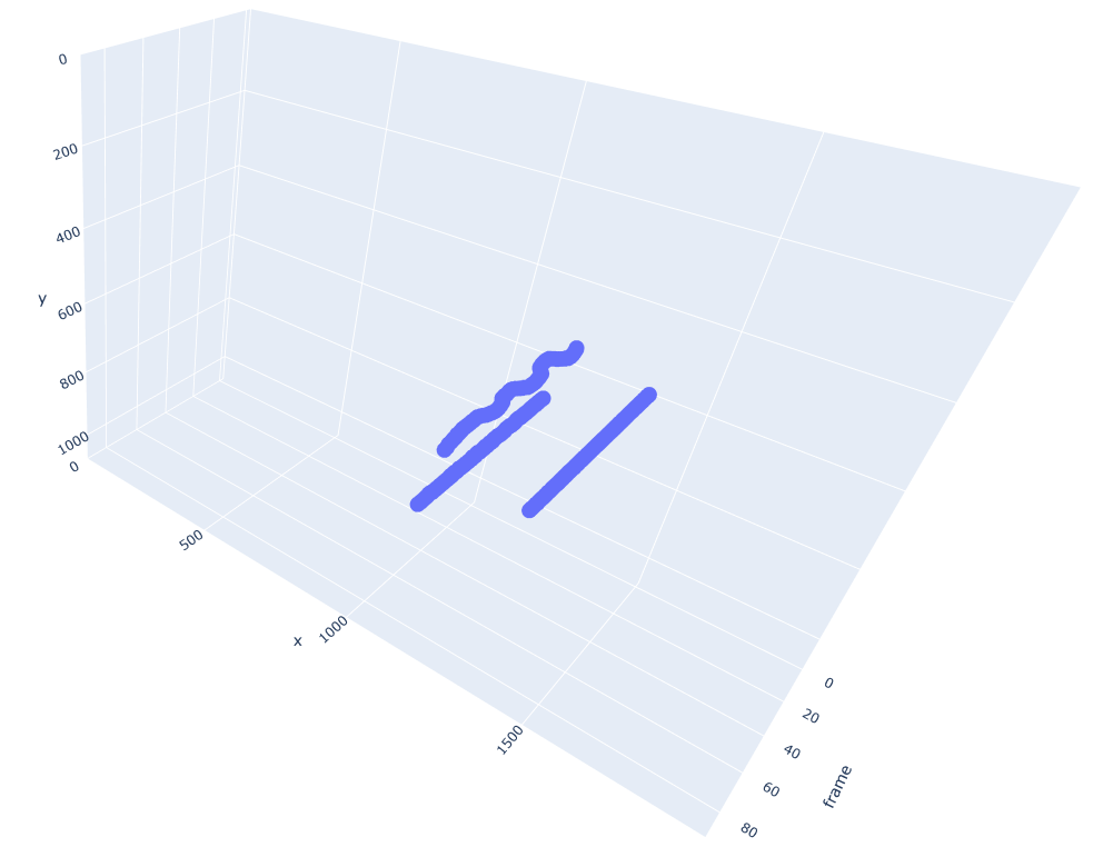
Figure 5: A three dimensional view of all balls and their positions within the first 90 frames of the sample video.

I then use the DBSCAN clustering model [7] from scikit-learn to cluster these points into distinct groupings as seen in Figure 6.

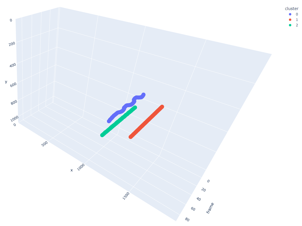
Figure 6: Three clusters identified using DBSCAN within the first 90 frames.

From here, we can separate the data into their respective clusters and find the active ball according to the cluster that has the most movement in the x & y dimensions. In the above example, this would be cluster 0.

From here, now that we know where the active ball begins, we add all other clusters to an exclusionary set that we deem as the “stationary balls” where we assume it is safe to say that any ball found within that region can be ignored in the future.

Linking Objects Between Frames

One interesting problem that I was faced with solving during this was trying to figure out the best way to store this data. I decided to go with a doubly linked list since I knew I had a series of frames that are all connected. In addition, I also had one object I called a trail that always kept track of the first and last nodes in the doubly linked list as seen below.

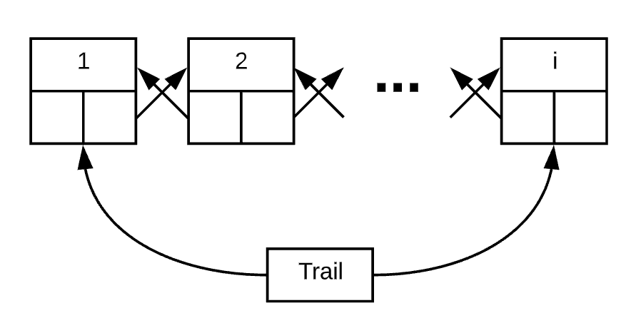
Figure 7: The doubly linked list data structure with an attached trail object used to keep track of the first and last nodes.

Storing the data this way allowed me to perform quick O(1) runtimes for all the functions that I would need quick access to.

Starting from the beginning of the video and the starting active positions given from the clustering performed earlier, I sequentially walk through the frames. For each new frame that I examine, I start by checking if any of the detected objects lie within range of one of the exclusionary set objects. If it is I can safely assume that that object is stationary and not active. This means that there are three cases that we need to account for given we have already excluded the existing stationary balls.

1. Zero balls are in the next frame.
2. Exactly one ball is in the next frame.
3. Two or more balls are in the next frame.

For the first scenario, we assume that either the model didn’t pick up the object or the ball has traveled to a location that can be seen by the camera (offscreen or behind someone). To remedy this, we leave the trail as blank for this frame and expand the search area for the next frame.

In any case besides the one just described; we perform the next two operations.

1. Predict where the ball should be based on the past X frames.
2. Determine the next active ball to be the one closest to the predicted or prior location.

The first step is performed through two independent quadratic regression models, one for the X value and one for the Y value. For both models, the frame number is used as the independent variable.

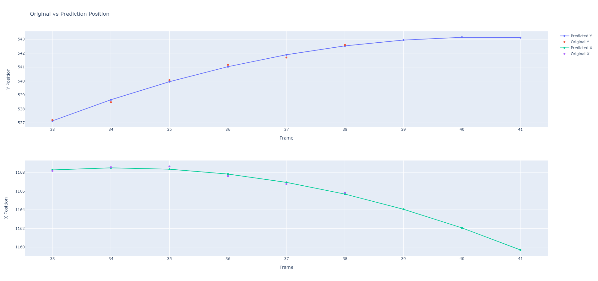
Figure 8: By fitting the regression model to the past X frames, we can predict ahead to estimate where the future location of the ball will be by combining the results of the x and y regression models.

Now that we have a predicted location, we can use that to narrow down which object is likely to be the active ball in the next frame. Any other ball that is not the closest one within this search area is then added to the exclusionary set. In practice, the model will sometimes pick up a random object in the middle of the video so this method helps with continuing to keep the exclusionary set up to date throughout the duration of the video.

Results

Putting all of this together, we can see in Figure 9 that this process works quite well to track the active ball throughout the duration of the video. As before, a link to a higher resolution video can be found on YouTube here. https://www.youtube.com/watch?v=3uQqHJMAisI

Figure 9: The tracked location of the active ball within the sample video with overlaying informational graphics.

Legend

• Blue Arrow: Active Ball Past Location
• Green Box: Active Ball Bounding Box
• Orange Open Circle: Active Ball Search Area
• Yellow Filled Circle: Predicted Active Ball Location
• Blue Box: Non-Active Ball Bounding Box
• Red Box: Net Bounding Box
• Red Circle: Exclusionary Set

In the parts of the video that are stuttering, that means that the model was not able to find anything that frame that was a part of the active ball set. This can also be seen by the expanded search area/orange open circle in some parts of the video. Over my testing, I found that a 6-frame lookback was sufficient to predict the location of the ball in the next frame. This might be able to be tweaked to get better results.

Reconstructions

In addition to this exported video, I created several other graphics that I thought were helpful in supplying additional information to the end results.

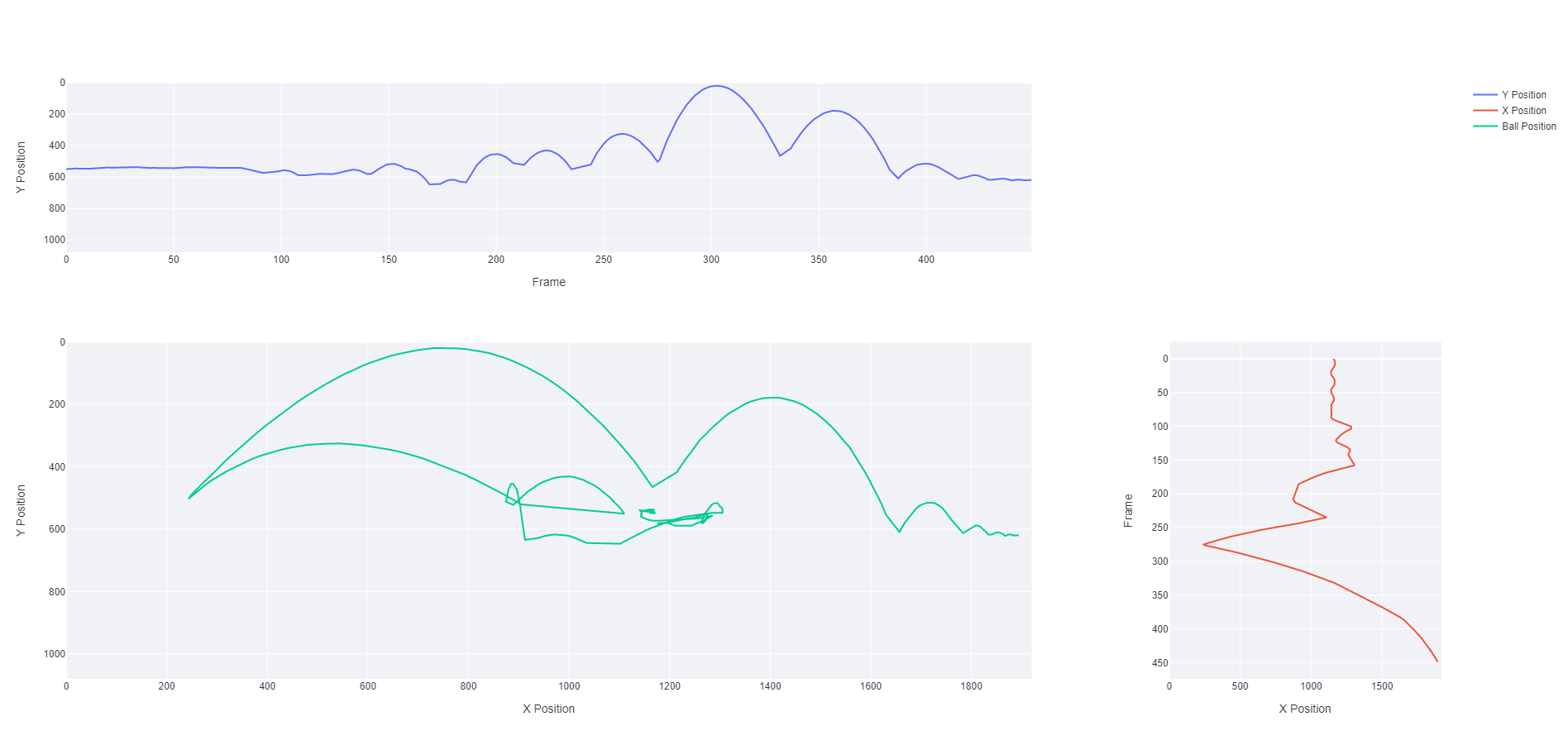
Figure 10: The active ball position tracked on a line plot. Both for over time in each respective dimension and once combined.

Figure 11: A 3D reconstruction attempt using a rolling average of the hypotenuse of the active ball’s bounding box as the Z dimension. The color of the scatter points corresponds to the frame number so that the darker colors correspond with earlier points in the video.

I was hoping that I could use the object detection’s consistency in predictions to use as an artificial measure for the Z dimension. However, as you can see from the 3D reconstruction, the depth suffers from many issues which stem from the fact that the bounding boxes that are given to the balls are already small. This gives an incredibly small margin for error and why you see the major arcs moving between the Z axis when it should be constant or linear.

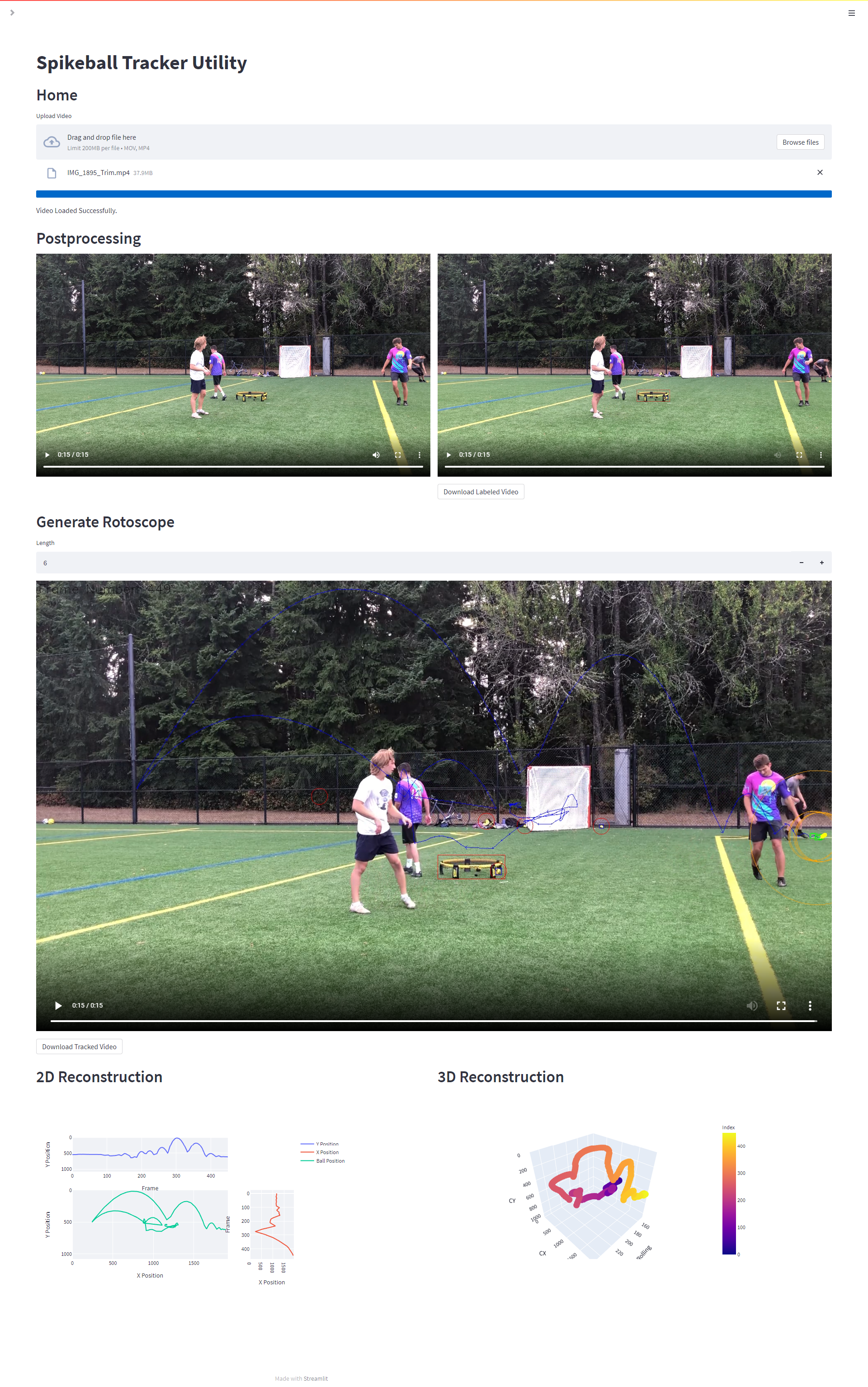
Application

Now that we have all the pieces built out separately, I wanted a seamless way to integrate each part with one another. Using Streamlit [8], I was able to create a local web application with Python where I could upload a video from my computer or other device connected via Wi-Fi and go through the same process in an automated fashion. A screenshot of that web app can be seen in Figure 12. And a YouTube video of the experience can be found here. https://www.youtube.com/watch?v=gk-UUunQf08

Improvements

As you might have been able to tell by now, the improvements made in this current version compared to the prior document shows immense progress in many of the areas that the pervious paper highlighted as limitations. Below are some of those major improvements.

• Generalizability: The major issue with the previous document was that everything described there was hand crafted for that specific video. With the steps outlined here, we have developed a generalizable model and pipeline that can be used on any roundnet footage that is commonly gathered.
• Standard Camera Position: The current method eliminates the need for a drone and instead utilizes the standard way for gathering this footage.
• Handel’s More Exceptions: We now can account for things like multiple balls in a frame, a hidden ball, lighting differences, and much more.
• Net Identification: Although the net was also identified in the previous version as well, it is also now more robust with the neural network.
• Better Python Programmer & Data Scientist: I myself have undergone a lot of personal growth over the past year which has allowed me to write better code and apply these deep learning concepts to this application.

Limitations

Everything isn’t sunshine and rainbows though. There is still a long way to go before a lot of the following limitations (some of which were raised in the prior document) will be completed.

• Speed: Although speed can be calculated, since we don’t have all three dimensions, the speed of the ball will be inaccurate.
• Depth: As seen above, there was an attempt to track the depth from the 2D video. However, this proved incredibly unreliable.
• Analytics: We are currently only tracking the ball, in order to track analytics, that means that we need to identify people, hits, and be able to track those for the duration of a game.
• Clipped Video: As you saw from the sample video, the methodology only works for one point during a game and the beginning had to be right when the player was about to server the ball. Forcing a user to clip each point after taking the video doesn’t make much sense and defeats the purpose of automation.
• Local Application: The Streamlit application worked great, however, it was only running on a local server on my machine where my graphics card could process the videos. This meant that I had to be on Wi-Fi in order to connect to it.

Recommendations

Below are some things that I have already began to think about as iterations for the next version of this project.

• Speed enhancements to make tracking and inferences perform in real time.
• Add linked tracking for a second camera setup to increase capture rate and allow for reliable multi-dimensional tracking. This could take form as a neural network that takes two camera video feed as input and can identify the same objects between both frames. However, I am unaware of any out of the box solutions currently available that could perform this analysis.
• Using image segmentation instead of bounding box-based object detection.
• Using a neural network that can track objects between frames of a video without having to manually search for links between frames.
• Tracking players and being able to continue to identify these players throughout the course of the video.
• Developing an app like the Streamlit proof of concept for commercial use.
• As stated above, there needs to be a way to upload the whole video to the pipeline without having to trim the video down for every point.
• Analytics as proposed by Roundnet Stats Tracker are a good beginning step to implement analytics where this application could be useful.
• Cloud computing would be necessary for performing these operations on a live app.

Conclusion

To conclude, throughout this document, we have explored a foundational implementation for machine learning in tracking key roundnet objects. Although we continue to have a long way to go towards getting an analytics engine running, the progress made up until this point proves instrumental for the potential success of this application in the future.

Future

This is not the end! I will continue to put work into this project and will continue working towards a future where a set of algorithms can automatically extract analytic metrics from roundnet footage. I will continue to work towards reducing the stated limitations and you will undoubtably hear from me again.

References

1. “NFL Next Gen Stats Powered by AWS”
2. “Tracking a roundnet ball from an Aerial View” Published 2020-03-31
3. “Detectron2: A PyTorch-based modular object detection library” Published 2019-10-10
4. “Husky Roundnet Club Instagram”
5. “Faster R-CNN: Towards Real-Time Object Detection with Region Proposal Networks” Published 2015-06-04
6. “Training a TensorFlow Faster R-CNN Object Detection Model on Your Own Dataset” Published 2020-03-11
7. “A Density-Based Algorithm for Discovering Clusters in Large Spatial Databases with Noise” Published 1996
8. “The fastest way to build and share data apps”